Simulation Setup

Video Tutorial

In this video tutorial, you will learn how to configure a Leda simulation file from scratch by adding structures, emitters, and detectors.

If the video cannot be played, try this: Alternate video link.

Main Interface

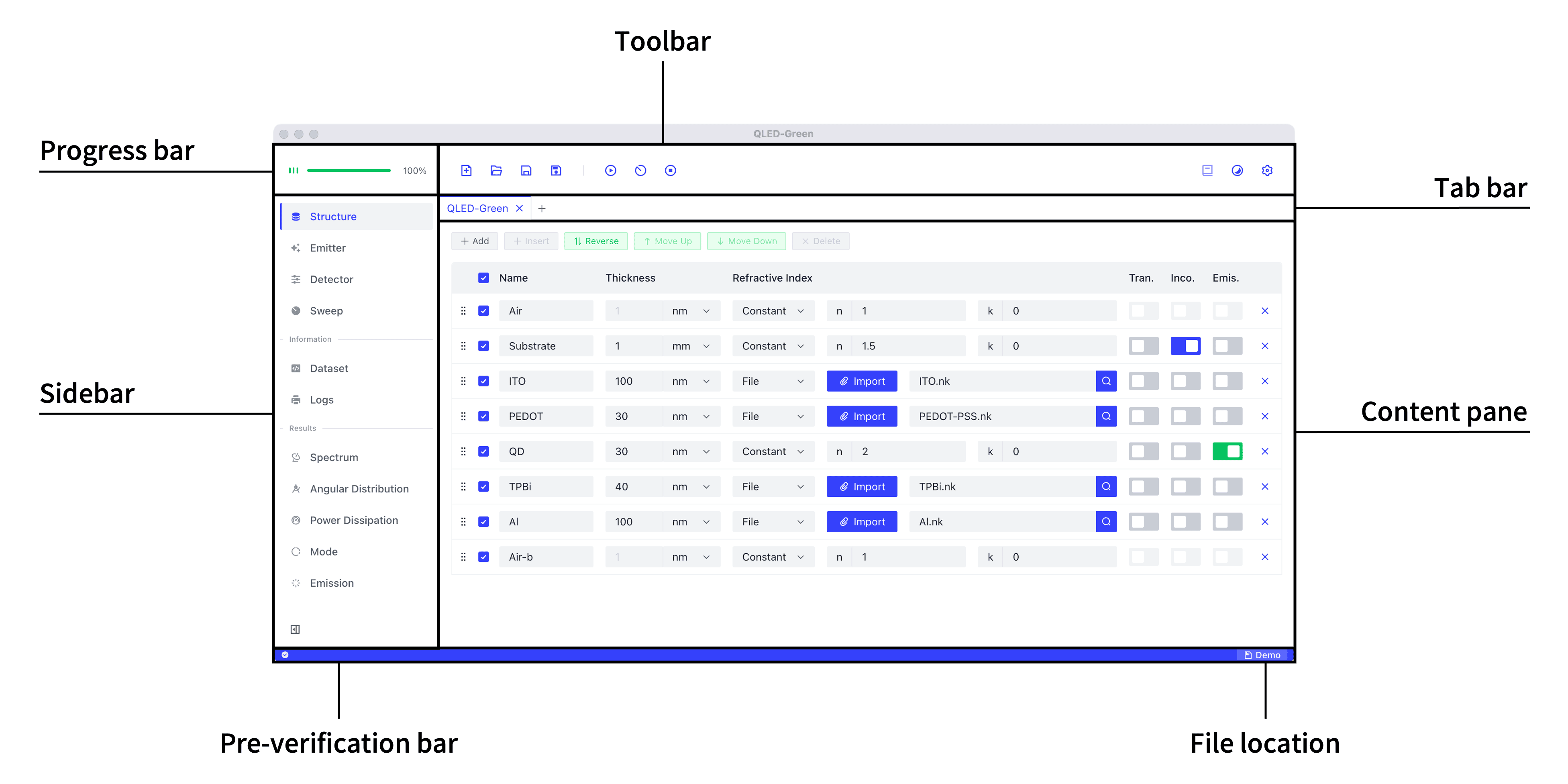
The main interface consists of the following modules:

• Progress Bar: Displays computation progress
• Toolbar: File operations such as open, save, run, and settings
• File Manager: Multiple open files are arranged in tabs
• Menu: Switch between configuration, information, and results
• Content Window: Set specific parameters and view simulation results
• Status Bar: Realtime error status and file location

Toolbar

The toolbar contains all the necessary functions for simulation (additional features such as opening a new window can be found in the top menu bar).

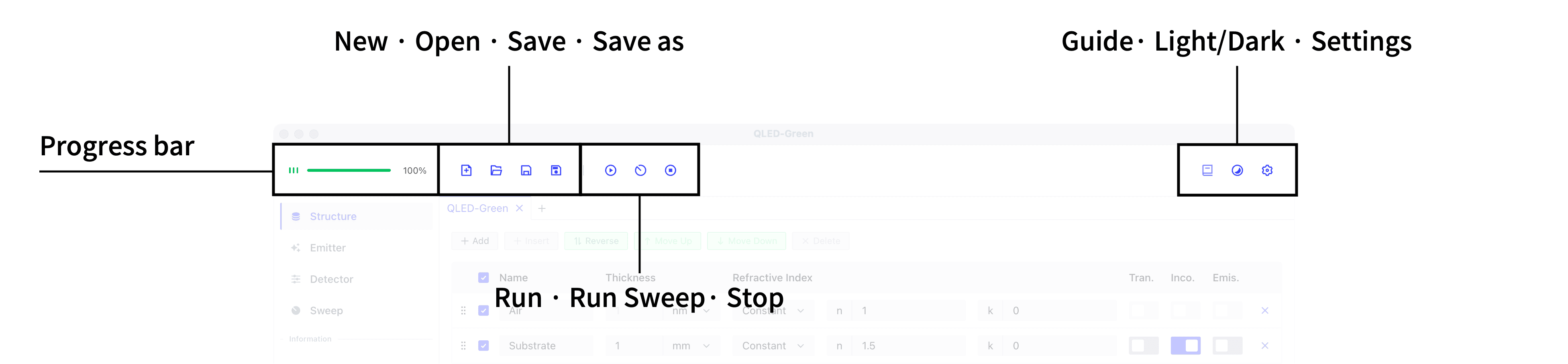
From left to right, the toolbar includes:

1. Progress Bar: The number of green dots on the left indicates the number of detectors that have completed simulation, while the overall progress is shown on the right. If an error occurs, the progress bar turns orange.
2. File Operations: New File, Open File, Save, Save As.
3. Simulation Operations: Run Single, Run Sweep, Terminate Run.
4. Manual (not yet supported), Light/Dark Mode Toggle, Settings.

Light/Dark Mode Toggle

The Light/Dark mode can follow the system setting or be manually toggled using the Light/Dark Toggle Button on the right side of the toolbar.

• For Windows, see Change colors in Windows for how to set system theme colors.
• For macOS, see Use a light or dark appearance on your Mac for how to set system theme colors.

Menu Bar

The top menu bar indicates shortcut keys for each function. Although the menu bar is used less frequently, it still contains some important features such as:

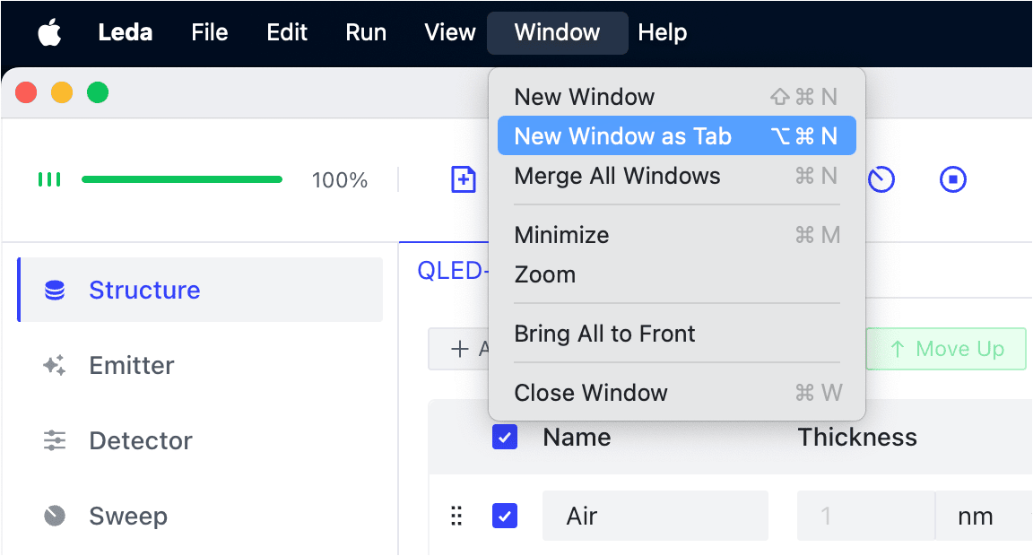
• Opening a new window, which can be used to compare results from two simulations.

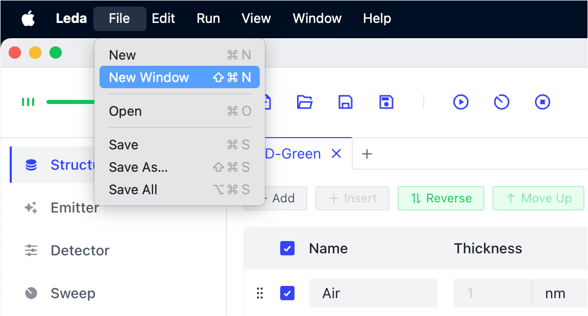
• Scaling the interface to optimize display on screens of different sizes.

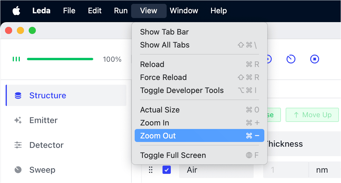
• macOS supports tabbed windows, while Windows can use software like Groupy for tab management of multiple windows.

File Management Bar

Multiple open files are arranged as tabs in the File Management Bar (Tab bar).

• New File: Click New in the toolbar, or click the Plus button in the File Management Bar.
• Create a new file on the right: For example, if files A and B are open and you want to insert C between A and B, right-click on A’s tab and click New to form the ACB tab order.
• Duplicate File: Right-click the tab of the file to be duplicated and click Duplicate.
• Close File: Click the ⨉ button to the right of the file name.
• Rename File: Right-click the tab and click Rename.
• Move Tab: Right-click the tab and click Move to Left or Move to Right.

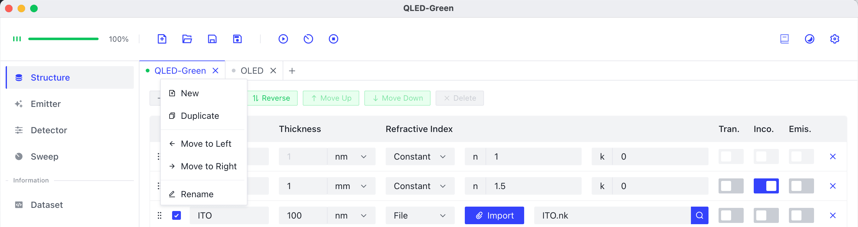
After modifying a file, a small dot appears to the left of the file name, which disappears after saving. Different colors of the dot represent different unsaved states of the file:

• Gray: No simulation results, not yet saved.
• Green: Successful simulation results, not yet saved.
• Orange: Failed simulation results, not yet saved.

Open in file management bar or new window?

Opening too many files in the File Management Bar may cause lag. For computers with insufficient single-core performance, it is recommended to open multiple files by creating new windows from the menu bar.

Sidebar

The left side of the interface is the sidebar. Clicking on a navigation item switches the content window to the corresponding section.

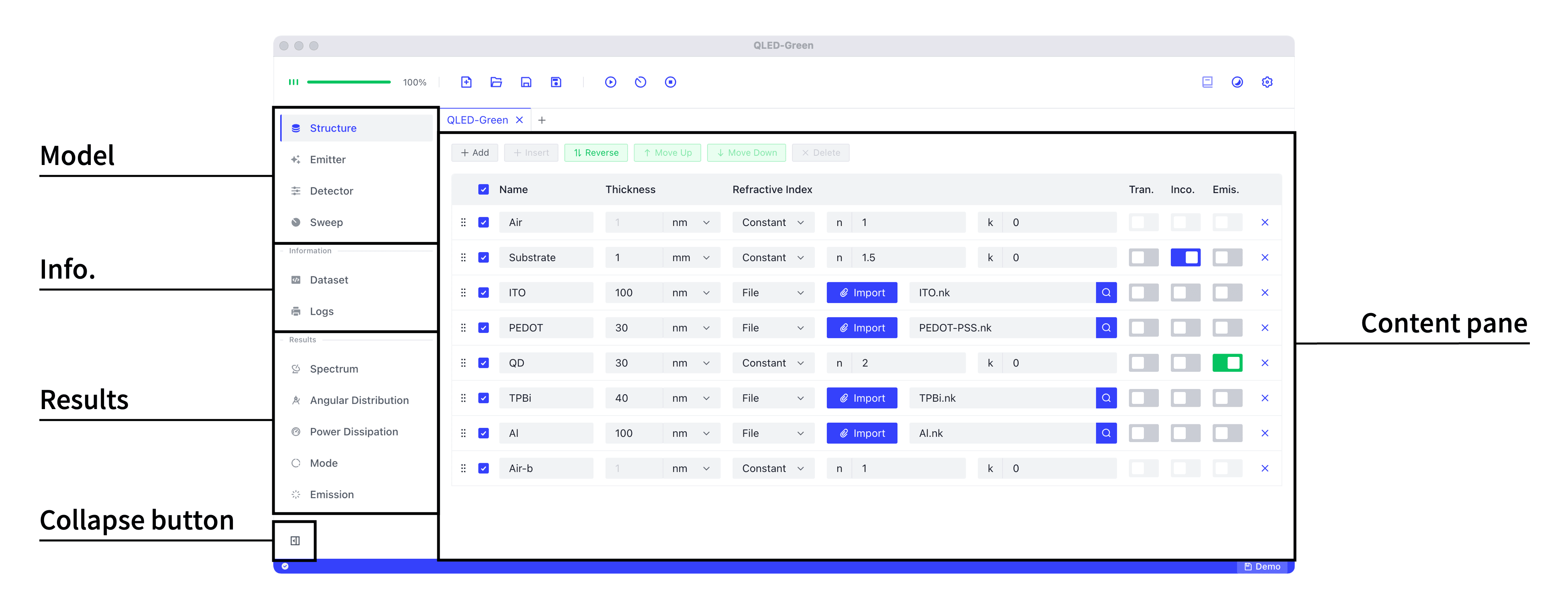
The sidebar is divided into three modules from top to bottom:

1. Modeling: Structure, Emitter, Detector, Sweep.
2. Information: Dataset, Logs.
3. Results: Spectrum, Angular Distribution, Power Dissipation, Mode, Emission.

If the content window is not fully displayed due to limited screen size, you can collapse the sidebar by clicking the button in the lower-left corner.

Settings

Click the Settings button at the far right of the toolbar to open the settings window.

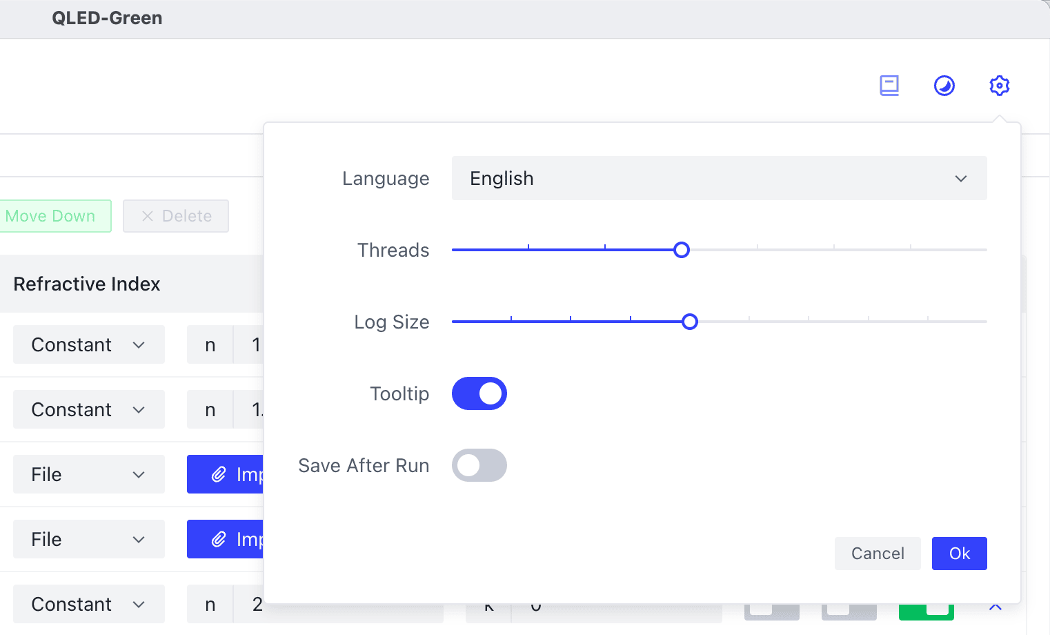
The following settings can be configured:

• Language: Supports English and Simplified Chinese. Not all terms have translations, so it is recommended to use English.
• Threads: Leda supports multi-threaded computation during sweeps. As modern computers generally have hyper-threading technology, setting it to half the available threads usually achieves optimal speed. Setting too many threads may actually reduce speed. If the computer lags during computation, further reduce the number of threads. The software needs to be restarted for thread settings to take effect.
• Log Size: Logs record the status and error information of each run. A new log entry is added for each run, and when the number of logs exceeds the set value, the earliest logs are automatically deleted.
• Tooltip: When enabled, hovering the mouse over a button or question mark icon displays a tooltip. If you are familiar with Leda operations, you can disable tooltips to reduce visual clutter.
• Save After Run: When enabled, files are automatically saved after each run.

Click Ok to apply the settings, or Cancel to discard changes.

Structure

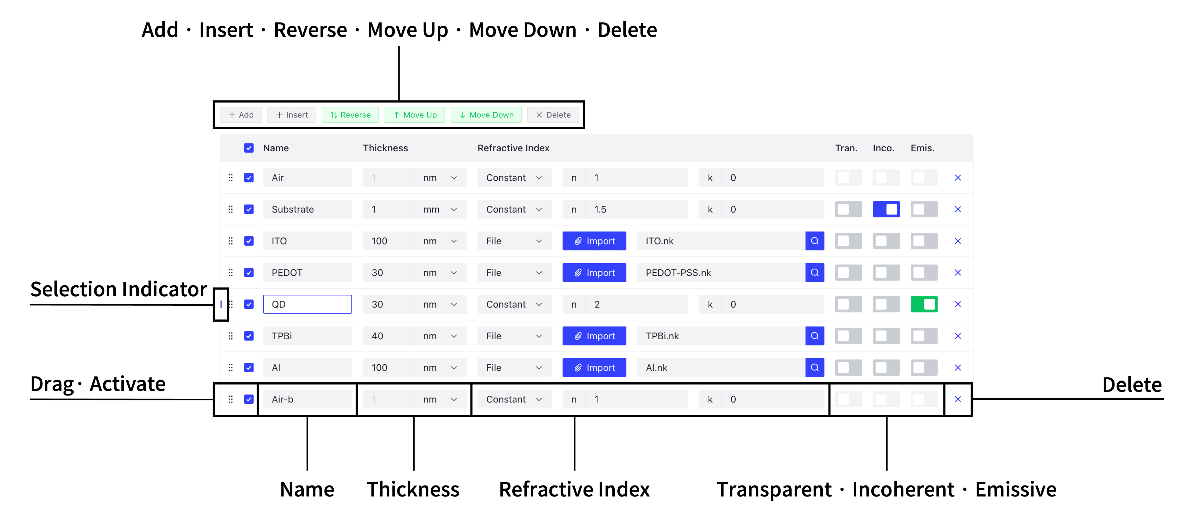
Click Structure in the menu bar to enter the structure configuration, where the content window displays as follows.

Building the Structure

At the top are structure operation tools, we can add, insert, move up, move down, and delete layers.

Insert, Move Up, Move Down, and Delete are unavailable until a layer is selected. To select a layer, click on its name, after which a blue selection indicator appears on the left of the selected layer.

• Adding a Layer: Click Add to add a layer at the bottom, or Insert to add a layer below the selected layer.
• Sorting Layers: Besides using Move Up and Move Down on a selected layer, you can also drag the ⋮⋮ symbol on the left to sort. Click Reverse to invert the order of the structure.
• Deleting a Layer: Select a layer and click Delete to remove it, or click the ⨉ on the far right of the layer.

Layer Order

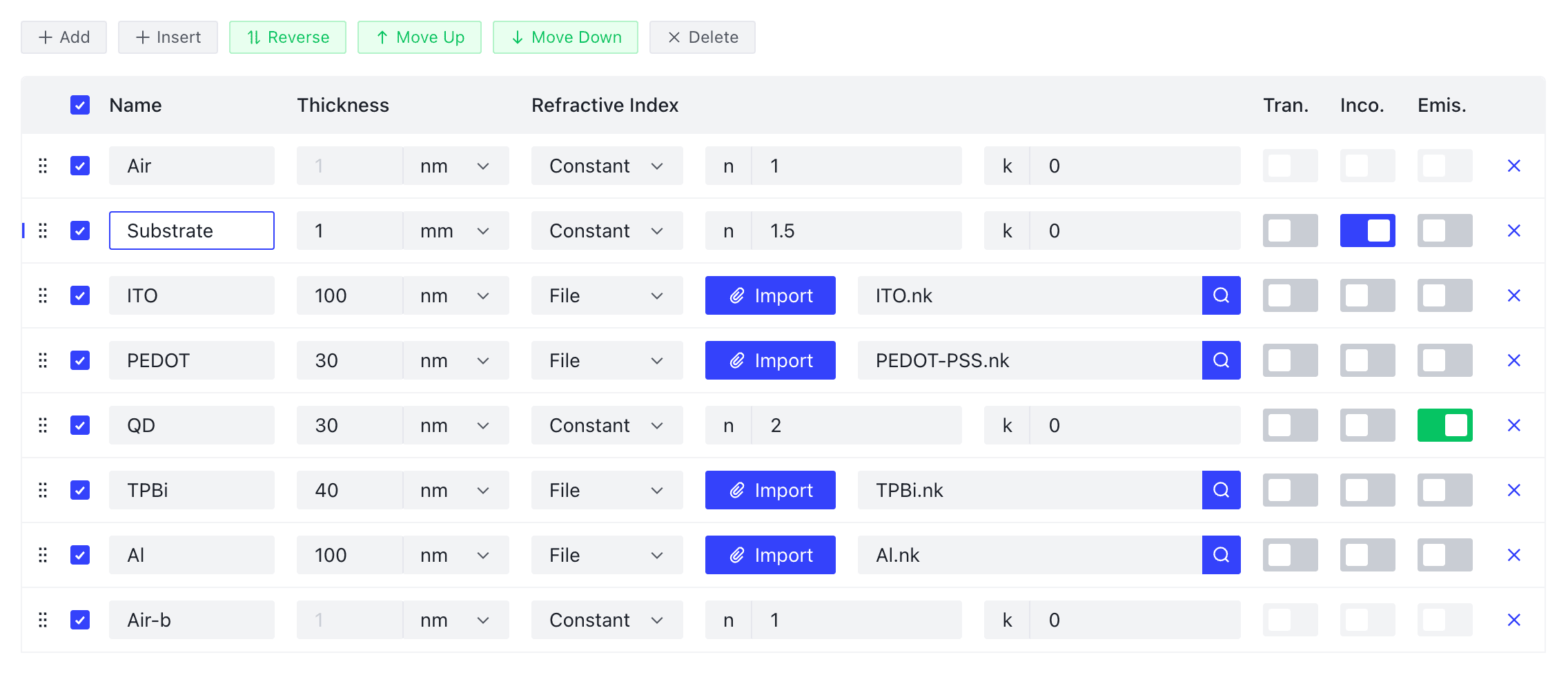
Whether your structure is top-emitting or bottom-emitting, the structure should be modeled with the light-emitting side facing upward. For example, in the bottom-emitting QLED structure, light is emitted from the substrate. Therefore, the first layer from top to bottom is air (the detector’s environment), followed by the substrate, and then other functional layers.

For a bottom-emitting structure like Substrate/ITO/PEDOT/QD/TPBi/Al, the substrate should be modeled facing up.

Correct order:

Incorrect order:

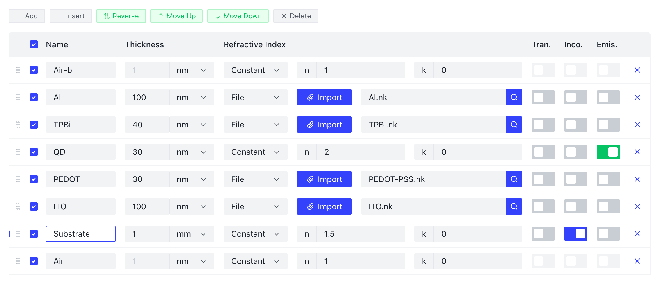
If the light-emitting surface is accidentally modeled facing down, click the Reverse button in the operation tools to invert the structure order.

In top-emitting structures, the substrate is often not the light-emitting surface, so it is modeled facing down.

The first and last layers in the model are semi-infinite in thickness, so their thickness cannot be set. Even if a thickness is set, it is treated as infinite; regardless of whether the transparent (Tran.) and incoherent (Inco.) properties are activated, they are treated as transparent and incoherent. These layers are generally set as air.

Layer Properties

• Name: Layers’ name must be unique.
• Thickness: Default unit is nm.
• Refractive Index options include:
  • Constant: Set the real part n and imaginary part k of the refractive index.
  • Constant Birefringence: Set the birefringence n_o k_o and n_e k_e.
  • File: Import refractive index files (supports birefringence). After import, click the magnifying glass icon ⚲ to view the refractive index chart.
• Transparent (Tran.): If a layer is set to transparent, its imaginary refractive index is set to 0 during computation.
• Incoherent (Inco.): Incoherent means that light does not interfere when propagating within this layer. Generally, thicker materials can be considered incoherent, such as a 1 mm thick glass substrate. Incoherent layers require that their surroundings are also incoherent, meaning a incoherent layer cannot be inserted between two coherent layers.
• Emissive (Emis.): The emissive property needs to be activated for an emitting layer. When Emis. is activated, the layer is treated as transparent regardless of whether its Tran. property is activated.

Incoherent Layer Considerations

1. Generally, only the substrate is set as incoherent.
2. An incoherent layer cannot be inserted between two coherent layers.

If light cannot reach the substrate (top-emitting structure), consider removing the substrate layer.

For example, in a top-emitting structure Air/Glass/Al(100 nm)/ETL/EML/HTL/ITO/Air, light can hardly penetrate the 100 nm thick Al to reach the Glass. In this case, it is recommended to remove the Glass layer.

Since Glass, as an incoherent layer, extends the calculation boundary of the Absorption mode’s to the refractive index of Glass, light reflected at the Al surface within is counted as Absorption mode.

Although this calculation does not affect other Modes, most researchers do not delve into how the Absorption mode is calculated, which may lead to a misunderstanding that the device has high absorption loss. Therefore, by simply removing Glass, this portion of energy is classified as Waveguide mode, making it easier for most researchers to understand.

For multi-layer incoherent structures, it is not recommended to use Leda

If the structure contains multiple incoherent layers, or each layer is tens of micrometers thick, using Leda is not recommended.

In such cases, strictly considering coherence in Leda leads to numerous interference fringes. However, the actual device will not have such a perfect coherent environment, causing discrepancies between simulation and experiment. If coherence is completely ignored and every layer is set as incoherent, there is no need to use Leda.

Leda relies on coherence to calculate microcavities and the various optical effects induced by them. If your device does not have microcavities or significant interference, consider using other simulation software.

Refractive Index Data Structure

If you want to import custom refractive indices, the data must adhere to the following format specifications:

• Columns are separated by spaces or tabs. Data copied from software like Excel or Origin is often already tab-separated.
• Comment lines start with # and are not read as data.
• Refractive index data files should have .txt or .nk as file name suffixes.

Standard refractive index data format: Wavelength (nm); real part of refractive index n; imaginary part k

Al.nk

# wavelength n k
300 0.2169982 2.982331
310 0.2314807 3.092004
320 0.2441945 3.198823
330 0.2575465 3.305539
340 0.2716037 3.412406
350 0.2900822 3.54058

Birefringence data format: Wavelength (nm); ordinary light (o-light) real part n_o; o-light imaginary part k_o; extraordinary light (e-light) real part n_e; e-light imaginary part k_e. Birefringence data requires the optical axis to be perpendicular to the interface.

TPBi.nk

# wavelength no ko ne ke
400.92 1.9556 2.37E-06 1.6434 0.00029767
402.51 1.9529 1.96E-06 1.6423 0.00026604
404.09 1.9502 1.63E-06 1.6413 0.00023776
405.68 1.9477 1.36E-06 1.6403 0.00021248
407.26 1.9452 1.14E-06 1.6393 0.00018988
408.85 1.9427 9.59E-07 1.6383 0.00016968

Third-party refractive index data

When refractive index files are sourced from papers or databases, ensure the materials used in the experiment match those from which the refractive index data is derived.

For instance, ZnO and ZnMgO nanoparticles are often used as electron transport layers (ETL), but third-party refractive index data might be for bulk materials. The refractive index of CdSe bulk material is ~2.5, but for CdSe quantum dot layers, it is generally between 1.8–2.0.

Thus, importing the refractive index of nanoparticle layers using bulk material data can lead to significant errors. Even if the data source is also nanoparticle-based, different synthesis and preparation methods can result in varying refractive indices for nanoparticle layers.

Emitter

Click Emitter in the menu bar to enter the emitter configuration, where the content window displays as follows.

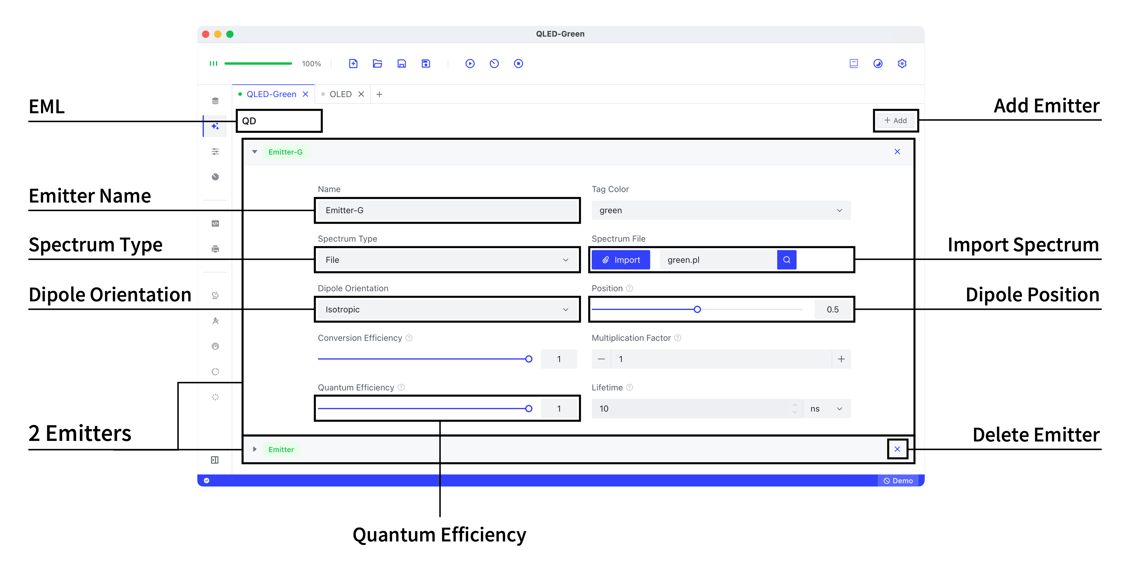
Layers with the Emis. property activated in the Structure will appear in the Emitter window. Previously, we activated the Emis. property for the QD layer, designating it as an emitting layer, thus its name appears in the upper left corner.

By default, an emitting layer has one Emitter. If more Emitters are needed, click Add on the far right of the emitting layer. The interface shows two Emitters.

Spectrum

Spectrum types can be selected as:

1. Unit White, which has the same intensity or photon count across all bands (not true white light).
2. File, import a spectrum file.

Spectrum files have .txt or .pl as file name suffixes, format: Wavelength (nm); Intensity or Photon Count.

red.pl

560 0.007972869
570 0.012127781
580 0.014351212
590 0.026358927
600 0.063194636
610 0.211850971
620 0.62964852
630 0.959306239
640 0.488650053
650 0.10278984
660 0.025351333
670 0.012790838

Spectrum units: Whether Unit White or imported spectrum, the vertical axis unit can be intensity or photon count. The simulated spectrum’s unit matches the input spectrum’s unit. If the imported spectrum’s vertical axis unit is intensity, then the simulated output spectrum’s vertical axis unit is also considered intensity.

Import PL spectrum instead of EL spectrum

The spectrum imported for the Emitter should be the photoluminescence (PL) spectrum, not the electroluminescence (EL) spectrum. EL spectrum is measured based on LED devices and is the result of optical effects within the device. Importing it into Leda for optical calculations would mean it undergoes optical effects twice.

Therefore, the intrinsic PL spectrum of the material, which has not undergone optical effects, should be imported.

Dipole Orientation

Dipole orientations include:

1. Isotropic, where dipoles oscillate in the x-y-z directions with equal weighting, meaning the same power is emitted in all directions. This is the choice for most emitting materials.
2. Parallel, where the oscillation direction is parallel to the interface, forming a horizontal dipole.
3. Perpendicular, where the oscillation direction is perpendicular to the interface, forming a vertical dipole.

Refer to: Dipole Approximation

Dipole Position

Range:

The position of the dipole within the emitting layer. A value close to 0 means the dipole is near the upper interface; a value close to 1 means it is near the lower interface.

Conversion Efficiency

Range:

Conversion efficiency unrelated to the radiation process, unaffected by the Purcell effect, such as the efficiency of electrical injection and the conversion of charges to excitons.

Refer to: Electrical and Non-Radiative Losses

Multiplication Factor

Range:

This factor amplifies the spectrum intensity by the corresponding multiple, typically used to adjust the relative intensity between multiple emitters.

Quantum Efficiency

Range:

Intrinsic quantum efficiency , also known as intrinsic radiative efficiency (RE). Quantum efficiency is affected by the Purcell effect.

Refer to: External Quantum Efficiency (EQE); Purcell Effect

Lifetime

Range:

Intrinsic lifetime of the dipole . Lifetime is affected by the Purcell effect.

Refer to: Purcell Effect

Detector

Leda includes three detectors:

1. Spectrum: Provides Spectrum and Angular Distribution results.
2. Power Dissipation: Provides Power Dissipation results.
3. Mode: Provides Mode and Emission results.

Click Detector in the sidebar to enter the detector configuration. Click the switch on the right of the detector to activate it. Multiple detectors can be activated simultaneously.

Spectrum

Expand the Spectrum detector to display as follows.

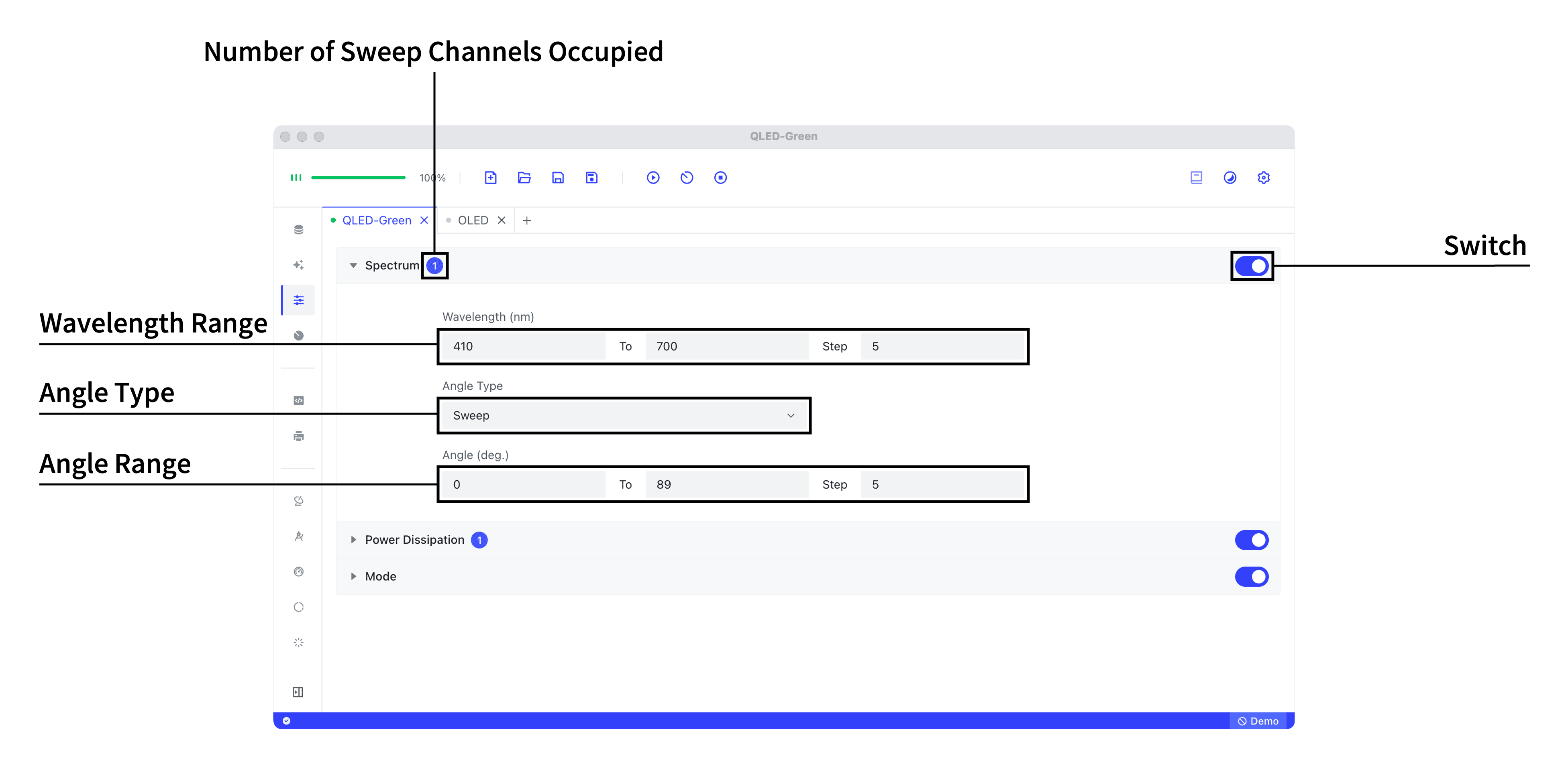
• Wavelength: Enter start value, end value, and step (nm).
• Angle Type:
  • Single: Outputs spectrum at a single angle in Results.
  • Integration: Outputs spectrum integrated over angles in Results.
  • Sweep: Angle sweep, occupying one sweep channel (a blue circle ❶ appears next to Spectrum). Outputs spectra at multiple angles and angular distributions at different wavelengths in Results.
• Angle:
  • When Angle Type is Single, enter a single angle (deg).
  • When Angle Type is Integration or Sweep, enter the starting value, end value, step (deg).

Power Dissipation

Expand the Power Dissipation detector to display as follows.

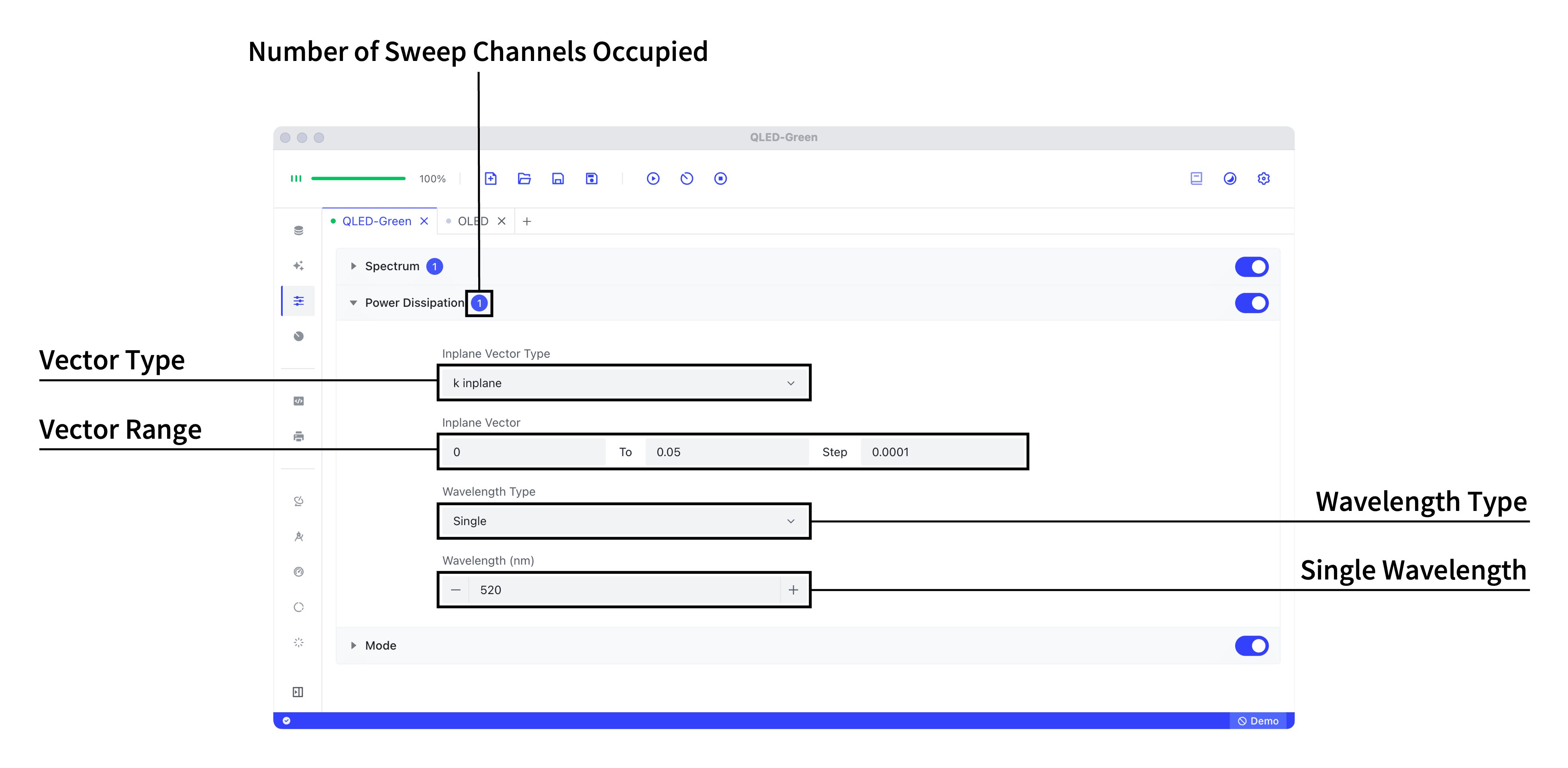
• Inplane Vector Type: Choose based on Power Dissipation.
  • k inplane
  • u inplane
  • n eff
• Inplane Vector: Enter start value, end value, and step.
• Wavelength Type:
  • Single: Single wavelength, occupying one sweep channel (a blue circle ❶ appears next to Power Dissipation).
  • Sweep: Wavelength sweep, occupying two sweep channels (a blue circle ❷ appears next to Power Dissipation).
• Wavelength:
  • When Wavelength Type is Single, enter a single angle (nm).
  • When Wavelength Type is Sweep, enter start value, end value, and step (nm).

How to set inplane vector range

Start Value is generally set to 0.

End Value is determined based on the type of inplane vector, wavelength, and refractive index of the emitting layer.

When light propagates parallel to the interface in the emitting layer, , ; , , the end value is recommended to be twice this value. For example, at a wavelength of 520 nm and a refractive index of 2.0 for the emitting layer:

• Set the end value for k inplane to .
• Set the end value for u inplane to .
• Set the end value for n eff to .

Step can be adjusted based on the end value, for example, calculating 200 points, step=(end value-start value)/200.

Dispersion relation and spectrum type

When Wavelength Type is Sweep, the Emitter’s spectrum is considered. If only exploring the dispersion relation of the structure, set the Emitter’s Spectrum Type to Unit White.

Mode

Expand the Mode detector to display as follows.

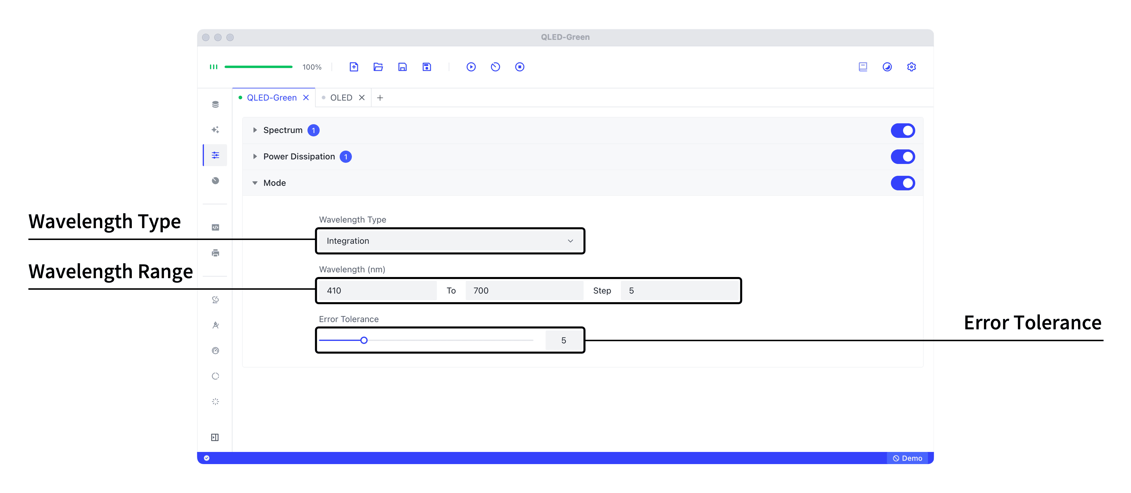
• Wavelength Type:
  • Single: Single wavelength.
  • Integration: Wavelength integration, simulation results are related to the Emitter’s spectrum.
  • Sweep: Wavelength sweep, occupying one sweep channel (a blue circle ❶ appears next to Mode). Simulation results are unrelated to the Emitter’s spectrum.
• Wavelength:
  • When Wavelength Type is Single, enter a single wavelength (nm).
  • When Wavelength Type is Integration or Sweep, enter start value, end value, and step (nm).
• Error Tolerance: Setting it to 5 is a low value, ensuring high simulation accuracy. If the simulation reports The result fails to converge in a finite in-plane wave vector, increase this value to allow results with larger errors. If set to 20 and the simulation still cannot solve, check if the settings meet the model’s conditions.

Mode detector error: the result fails to converge

Mode detector error: The result fails to converge in a finite in-plane wave vector.

Complete error:

The result fails to converge in a finite in-plane wave vector. Possible reasons: Dipole is placed too close to absorptive material or metal, or the refractive index of the emitting layer is too small. If there are no above problems, try to set larger Error Tolerance.

Cause analysis: This is due to the Evanescent (SPP) Mode region being too strong for the software to guarantee convergence, so it stops running early to prevent outputting results with a large error.

Try the following solution:

• Increase the distance between the dipole and the metal layer (increase the thickness of the transport layer), and if the thickness of the transport layer is sweeped, check that the From value is not too small.
• Change the metal material (Al/Ag/Au, etc. metal).
• Increase the Error Tolerance of the Mode detector (i.e., tell Leda to allow results to be output with a larger error)
• Adjust the wavelength range of the detector (a limited attempt could be made, as realistically the wavelength range may be required to be fixed)