Simulation Results

After completing the simulation setup, click the Run button in the toolbar. Once the simulation is complete, view the results in the Results section of the sidebar.

Spectrum

Click Spectrum in the sidebar to display the following.

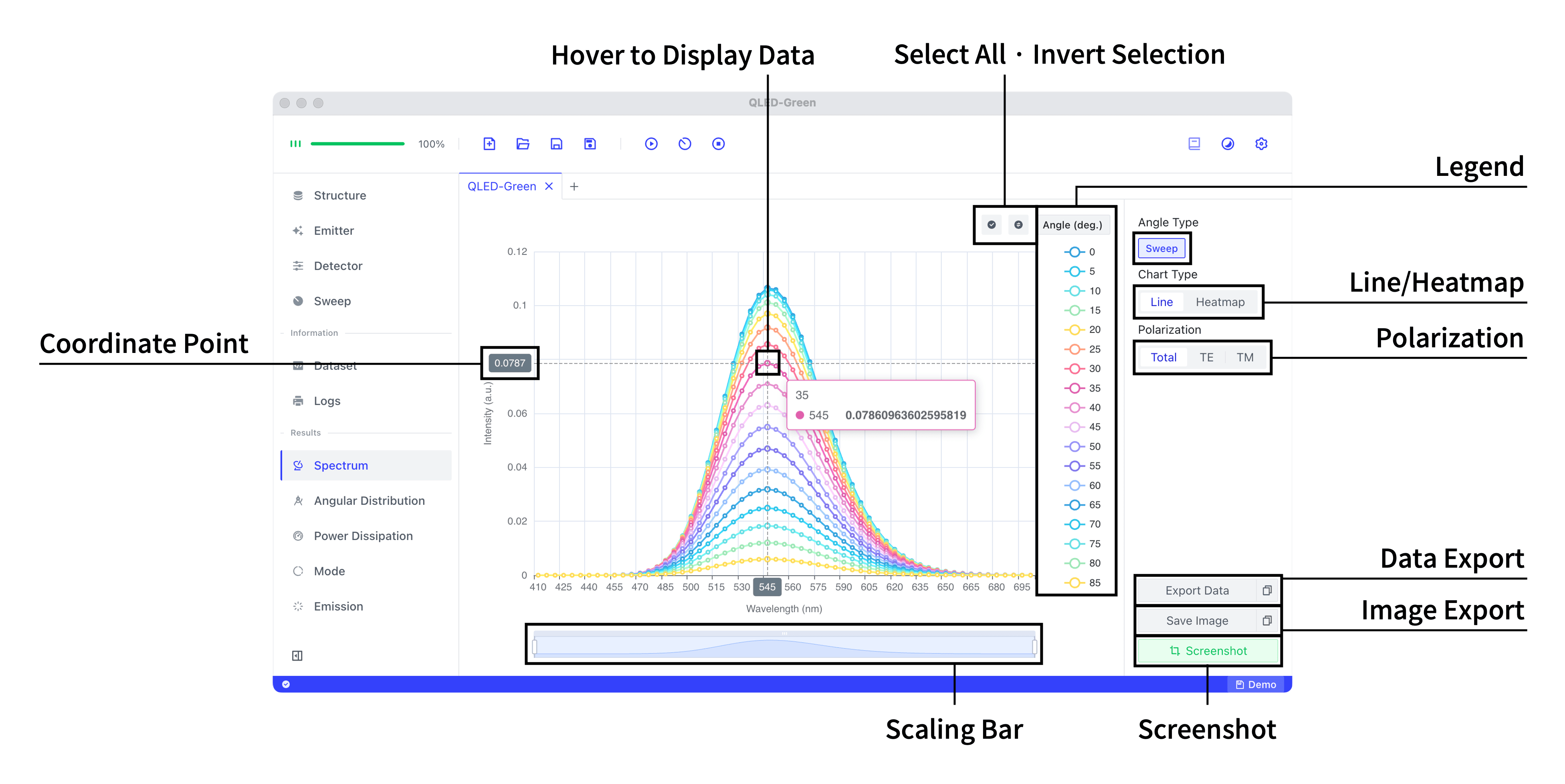
• Data Viewing: Hover over a data point to display its specific data.
• Zooming: Scroll the mouse wheel within the chart to zoom in and out; precise zooming can be achieved through the range zoom bar below.
• Data Selection: To display only certain data from the legend, click the data to deselect it, then click ⦾ to invert the selection.
• Chart Type Switching: Click Line and Heatmap under Chart Type to switch between line chart and heatmap.
• Polarization Switching: Click options under Polarization to switch polarization.
• Data Export: Click Export Data to save data locally; or click the ❐ on the right to copy data to the clipboard, then paste it into Excel or Origin for quick plotting.
• Image Export: Click Save Image to save the current image; or click the ❐ on the right to copy the image to the clipboard, allowing you to paste it into documents, emails, or IM software.
• Screenshot: The Screenshot button in the bottom right corner allows for screenshots with annotations, useful for quick sharing.

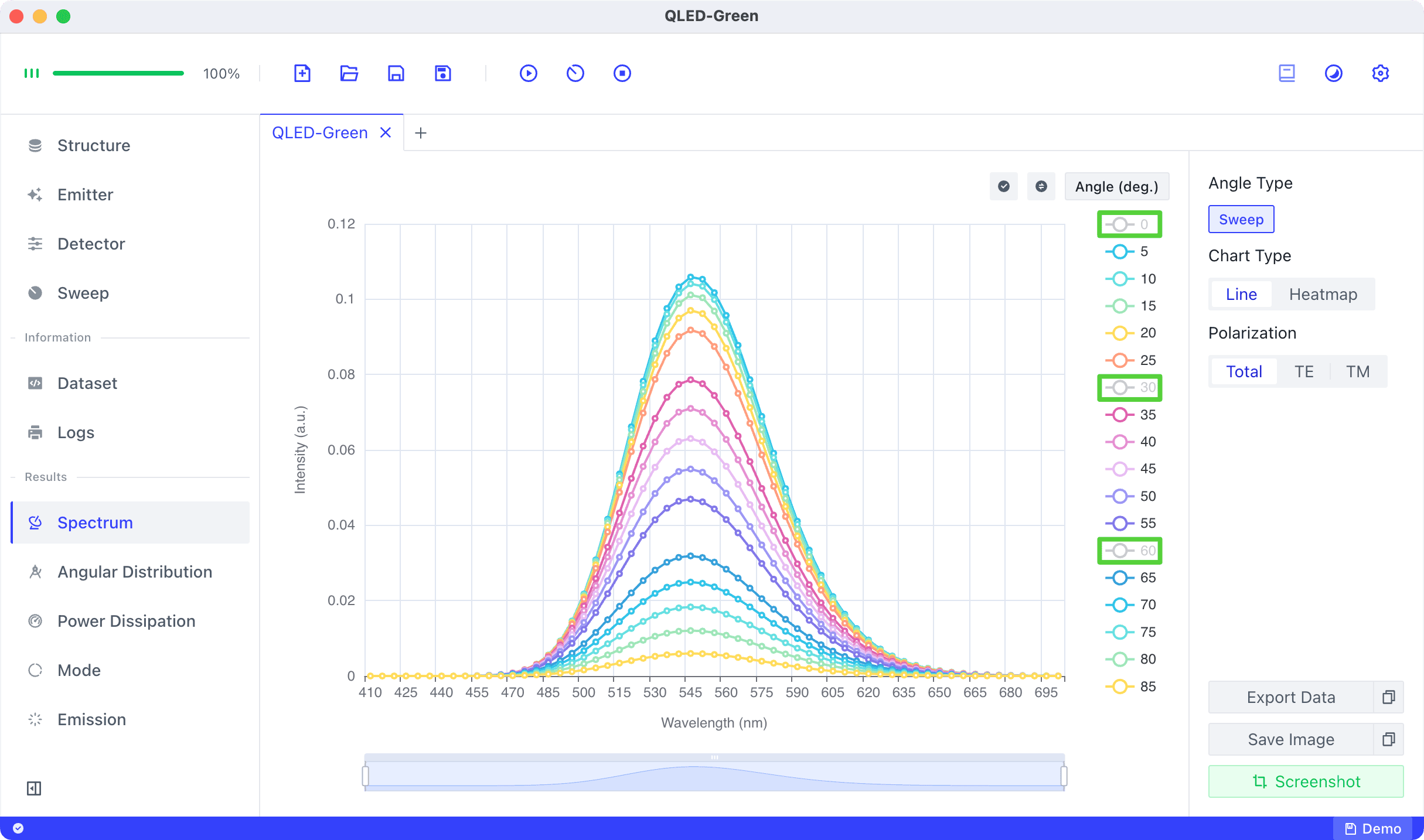
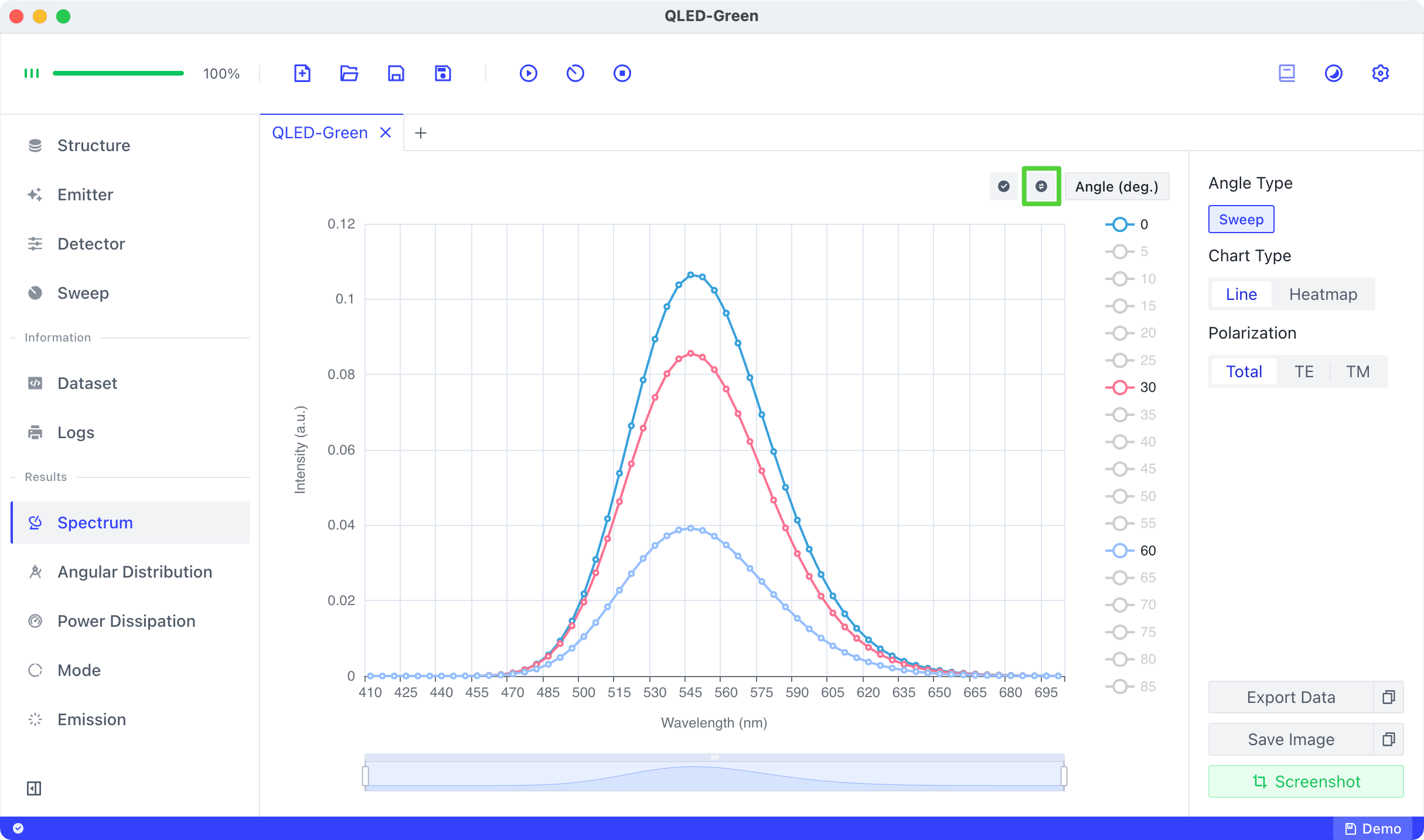
How to display spectra at 0, 30, and 60 degrees only

1. Deselect 0, 30, 60 in the legend.

   

2. Click invert selection to display only the spectra at 0, 30, and 60 degrees.

   

3. Click select all to return to the initial state.

Angular Distribution

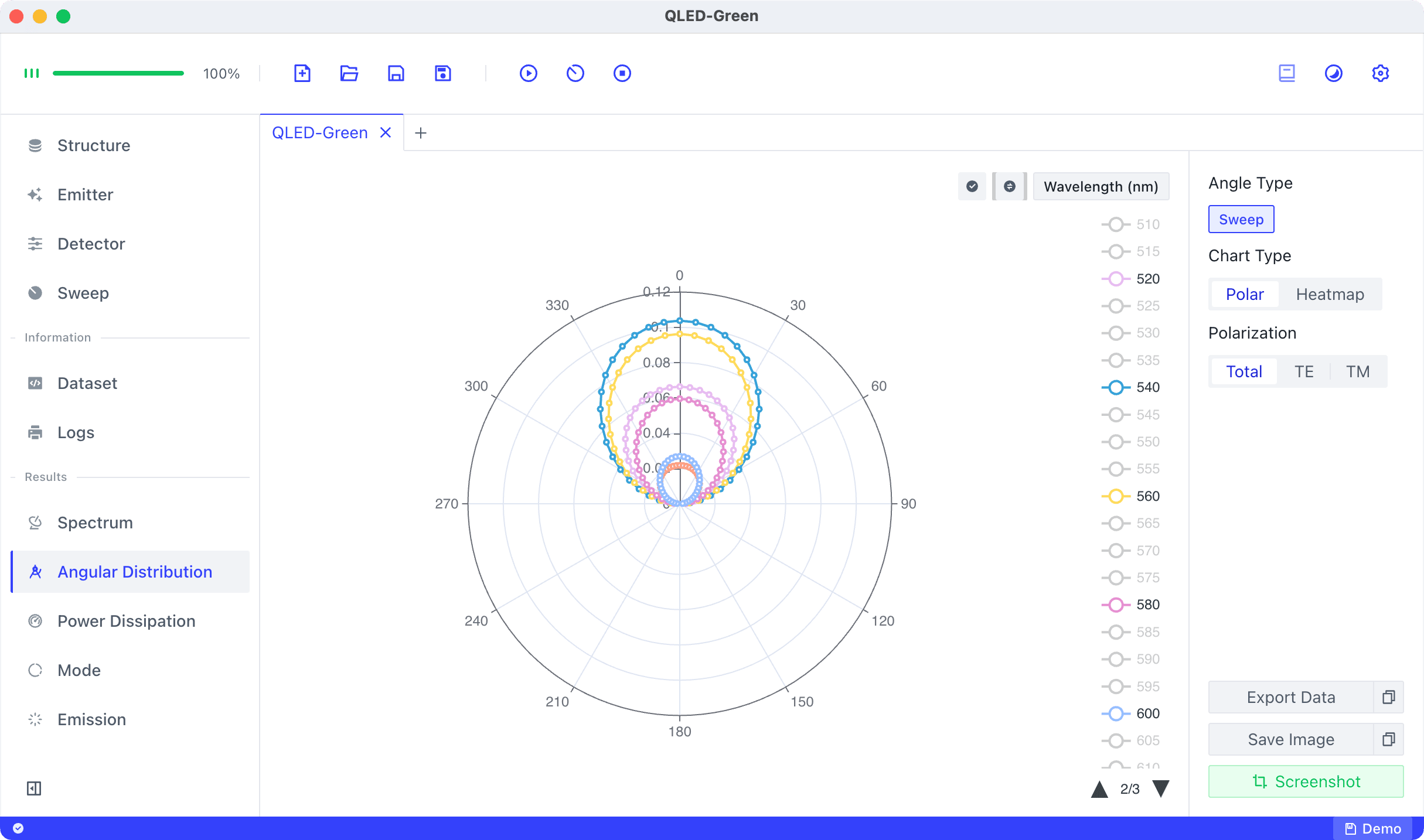
When Angle Type in the Spectrum detector is set to Sweep, the simulation outputs Angular Distribution results. Click Angular Distribution in the sidebar, and select wavelengths 500, 520, 540, 560, 580, 600 in the legend.

Power Dissipation

Click Power Dissipation in the sidebar. The current Legend is Direction, and Polarization is Total, displaying the following data:

1. Dissipated power of the sum of the TE + TM waves in the full plane wavevector range
2. Dissipated power of the sum of TE + TM waves into the top layer
3. Dissipated power of the sum of TE + TM waves into the bottom layer

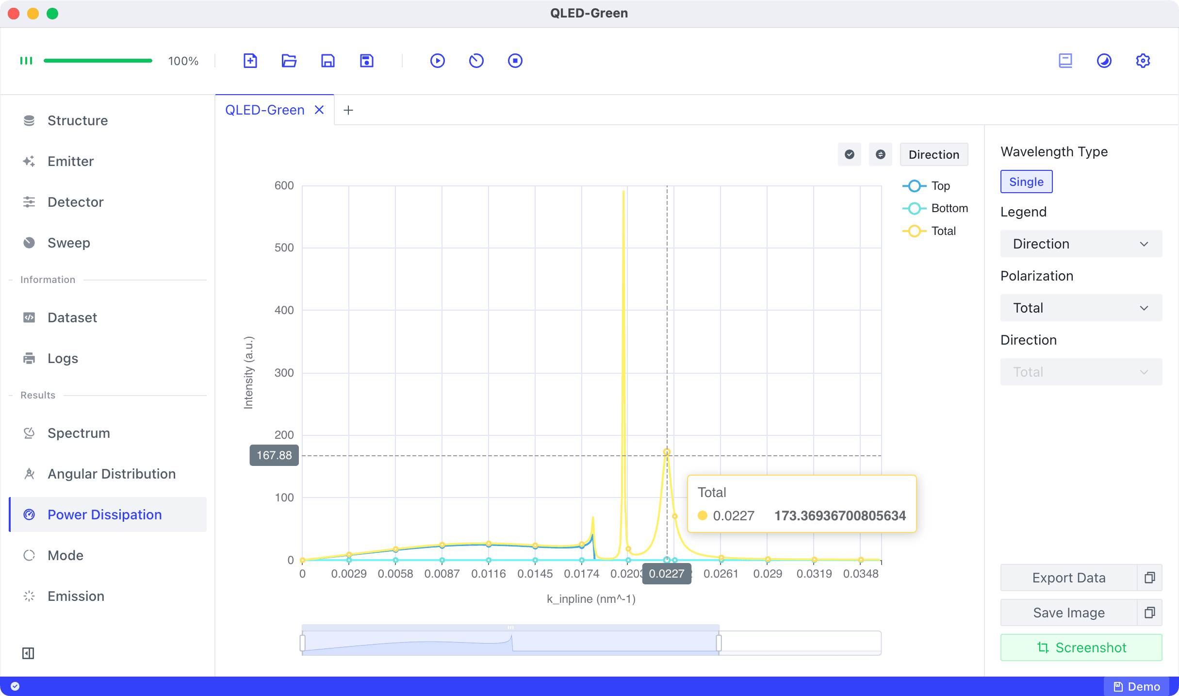
Right-side settings:

• Legend
  • Direction: Direction as the legend (default)
  • Polarization: Polarization as the legend
• Polarization (selectable when Legend is Direction)
  • Total: Displays the dissipated power of the sum of TE + TM waves (default)
  • TE: Displays only the dissipated power of TE waves
  • TM: Displays only the dissipated power of TM waves
• Direction (selectable when Legend is Polarization)
  • Total: Displays the dissipated power over the full in-plane wave vector range (default)
  • Top: Displays only the dissipated power entering the top layer (usually Air)
  • Bottom: Displays only the dissipated power entering the bottom layer (usually Air)

Switch Legend to Polarization, with Direction set to Total, displaying the dissipated power over the full in-plane wave vector range.

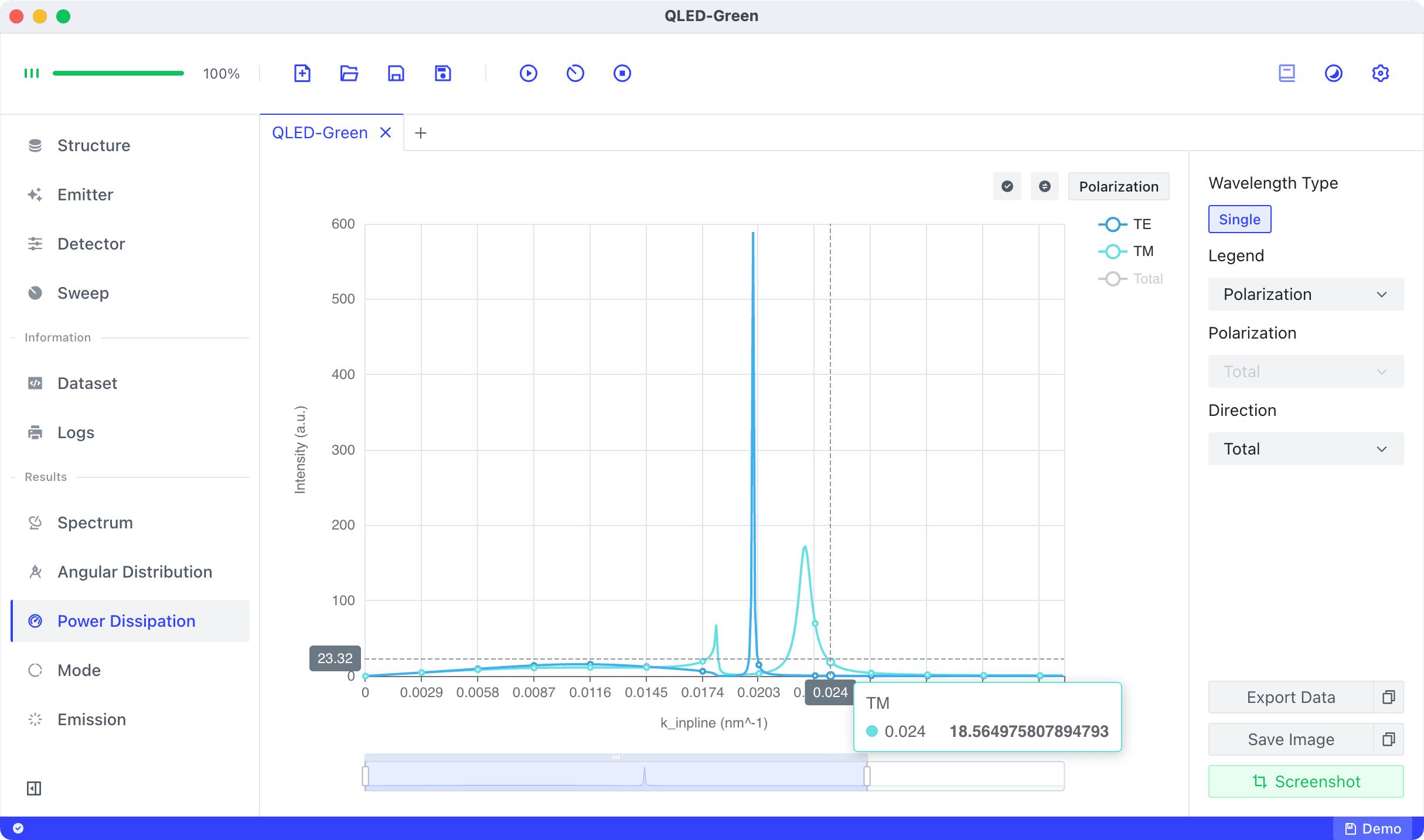
Given the current refractive index of EML is 2, with the Power Dissipation detector’s wavelength set to 520 nm, the boundary between Waveguide mode and Evanescent mode is . It is observed that TE waves generate strong constructive interference at in Waveguide mode, while TM waves primarily dissipate in Waveguide mode and cause minor dissipation in Evanescent mode.

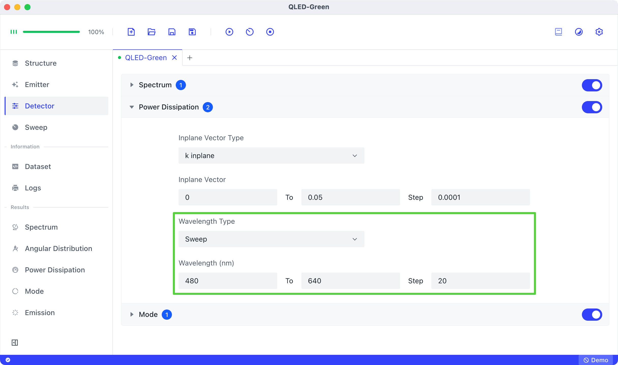
When the Power Dissipation detector’s Wavelength Type is set to Sweep from 480 to 640 nm with a step size of 20, the following is observed.

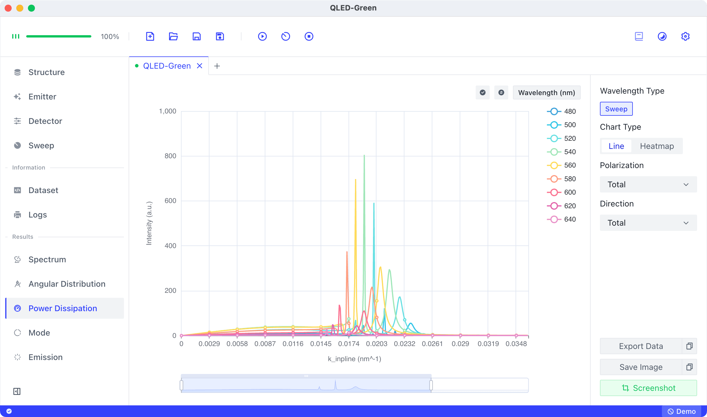
The simulation outputs Power Dissipation results at different wavelengths as follows.

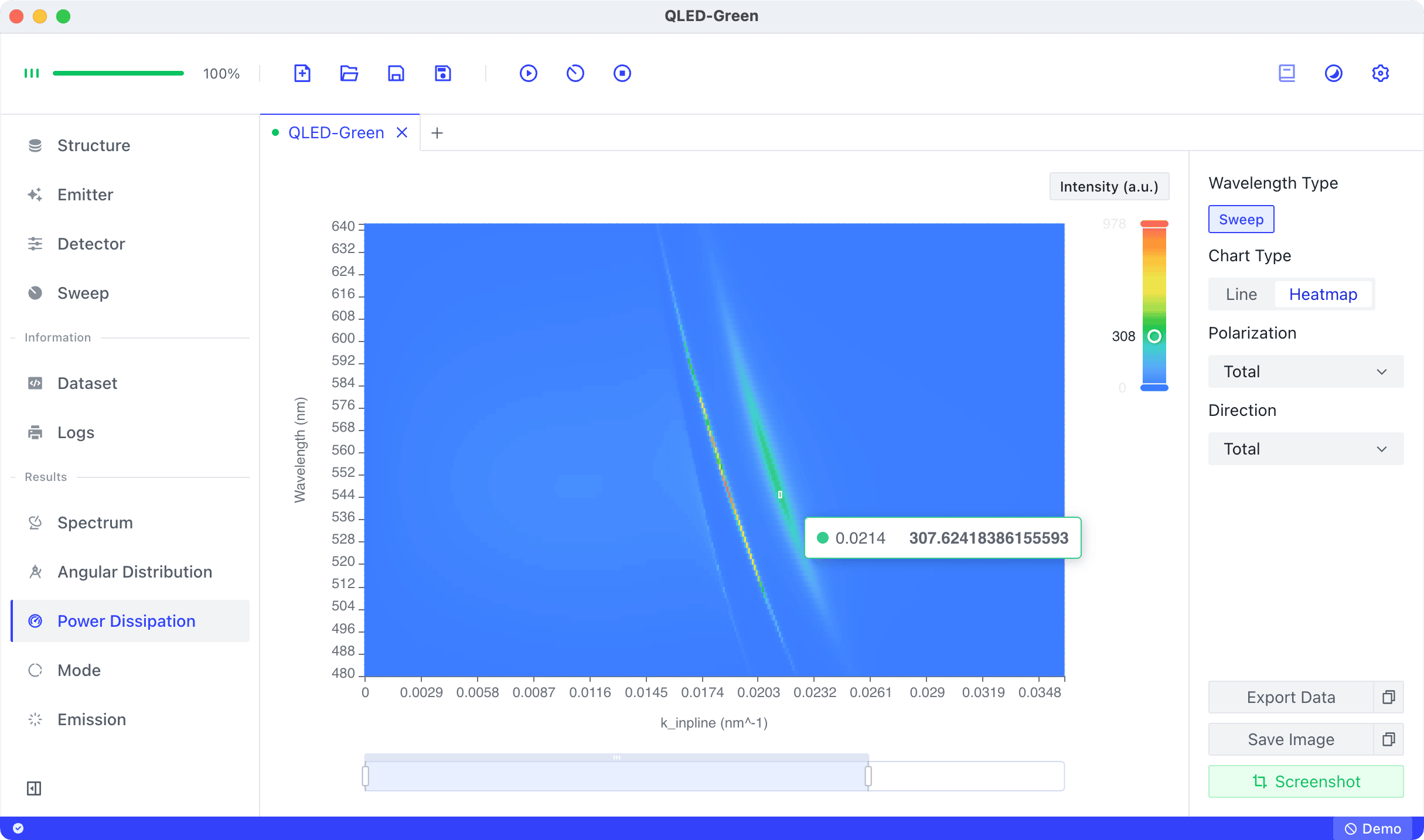
Reducing the step of the Power Dissipation detector’s wavelength to 2 can improve the precision of the wavelength sweep. In the simulation results, switch the Chart Type to Heatmap for a more intuitive view of Power Dissipation changes with wavelength.

Mode

Click Mode in the sidebar, and the Mode distribution is displayed as a doughnut chart showing the percentage of each Mode.

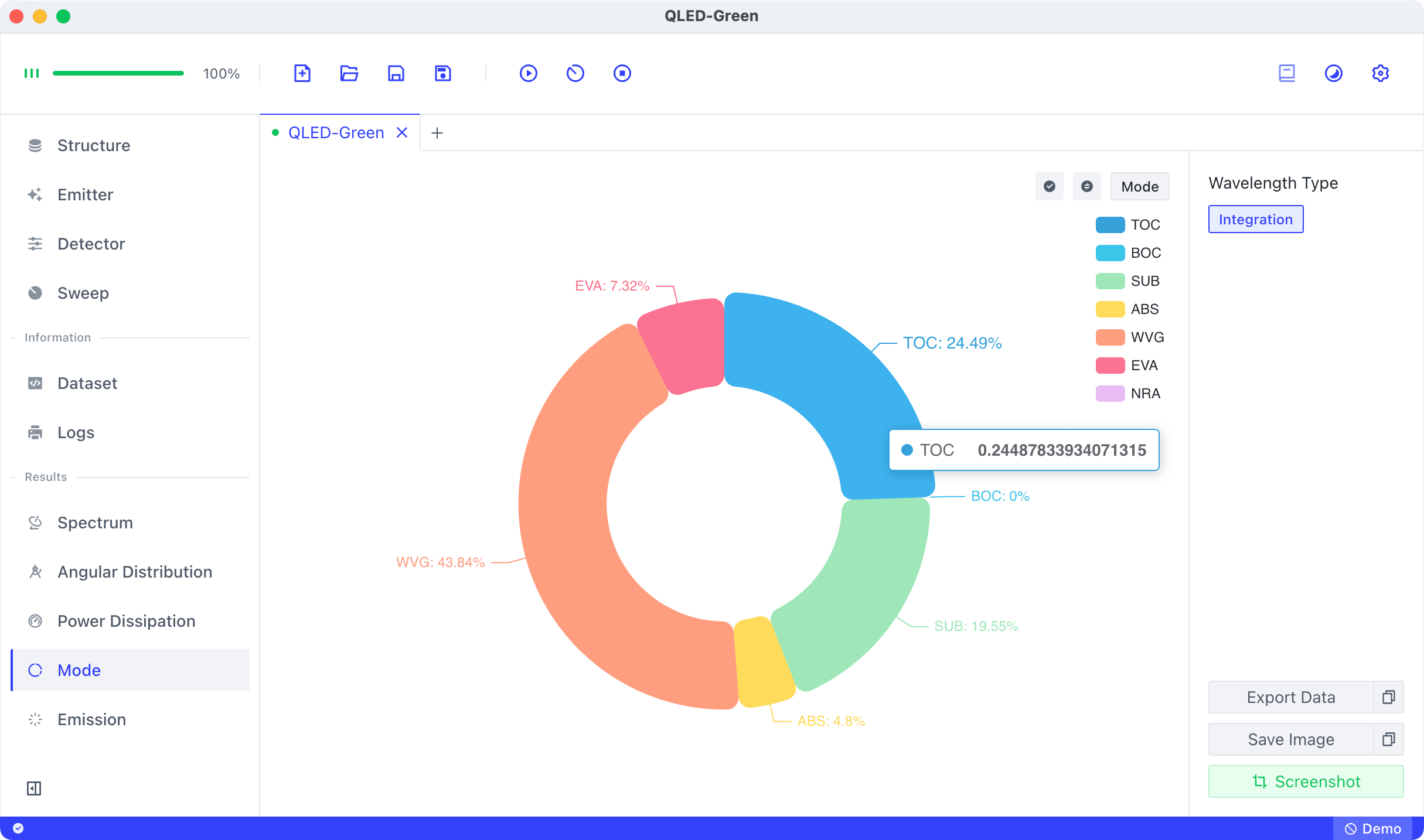
Since both Conversion Efficiency and Quantum Efficiency in the Emitter configuration are set to 1, TOC corresponds to EQE and LEE, at 24.49%. The main loss occurs in WVG (Waveguide mode), consistent with observations in Power Dissipation.

For definitions of each Mode in the chart, refer to: Optical Mode

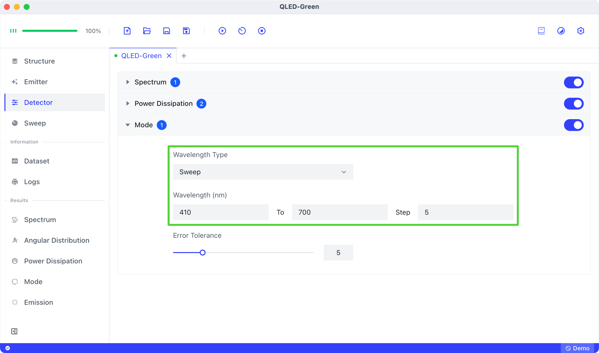
To explore Mode distribution at different wavelengths, set the Mode detector’s Wavelength Type to Sweep.

The following Mode results appear after running.

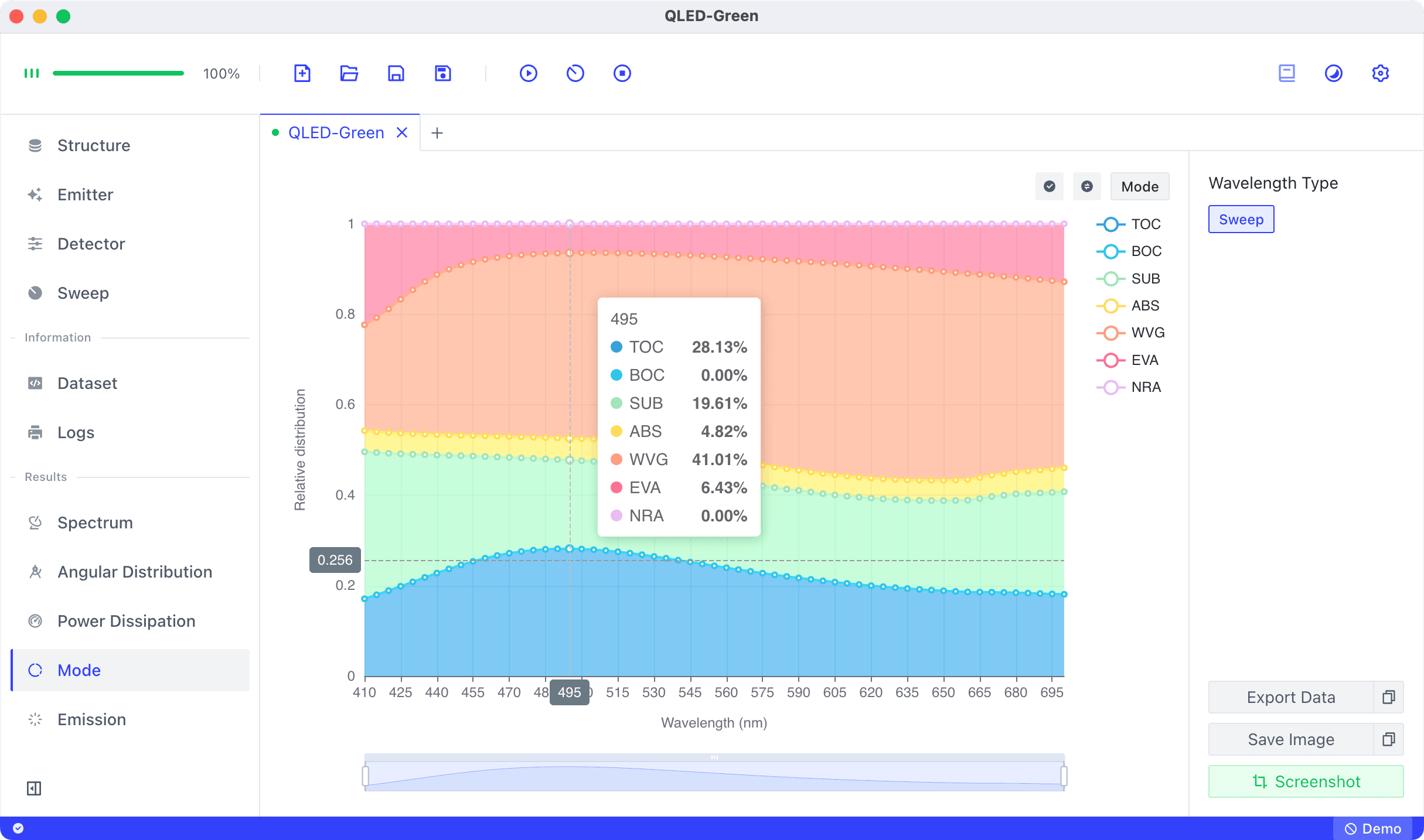
The simulation results show that the highest TOC value occurs at a wavelength of 495 nm, rather than our target wavelength of 520 nm. This indicates that although the device has achieved relatively good LEE, there is still room for optimization.

Are mode and spectrum related?

• When the Mode detector’s Wavelength Type is set to Sweep, the Mode results are unrelated to the Emitter’s spectrum. Because the Mode for each wavelength is calculated separately, the percentage of each mode does not change with spectrum intensity.

• When the Mode detector’s Wavelength Type is set to Integration, the Mode results are related to the Emitter’s spectrum. In this case, the Mode for each wavelength is calculated and summed based on the intensity weighting at different wavelengths, thus it is related to the spectrum.

When Conversion Efficiency and Quantum Efficiency in the Emitter configuration are not 1, NRA (Nonradiative mode) appears.

Set the Emitter’s Quantum Efficiency to 0.5, the Mode detector’s Wavelength Type to Integration, and rerun the simulation. The Mode results are as follows.

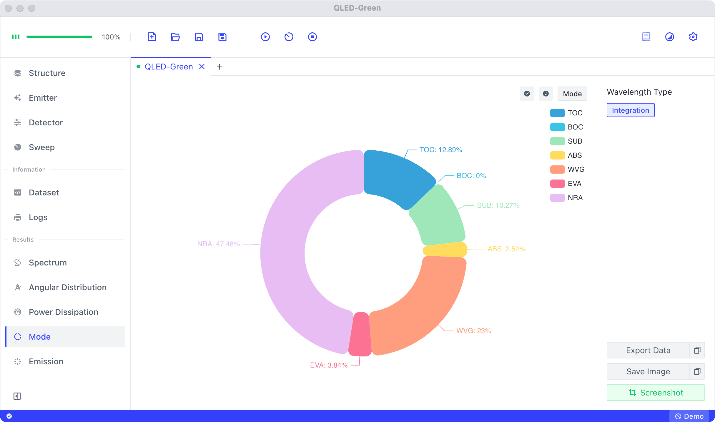
Although the intrinsic quantum efficiency is set to 0.5, the NRA percentage is 47.48% instead of 50%; the TOC percentage is 12.89% instead of halved to 12.25%. This is because the Purcell Effect enhances the effective quantum efficiency. Refer to: Purcell Effect.

Device structure influence IQE

This case illustrates that in addition to optimizing the emitting material to improve internal quantum efficiency (IQE), we can also regulate the Purcell factor through the device structure to achieve IQE enhancement.

Emission

Click Emission in the sidebar to view the emission properties of the Emitter. If there are multiple Emitters, you can view Emitters’ properties individually.

When the Emitter’s Quantum Efficiency is set to 0.5, the Emission simulation results are as follows.

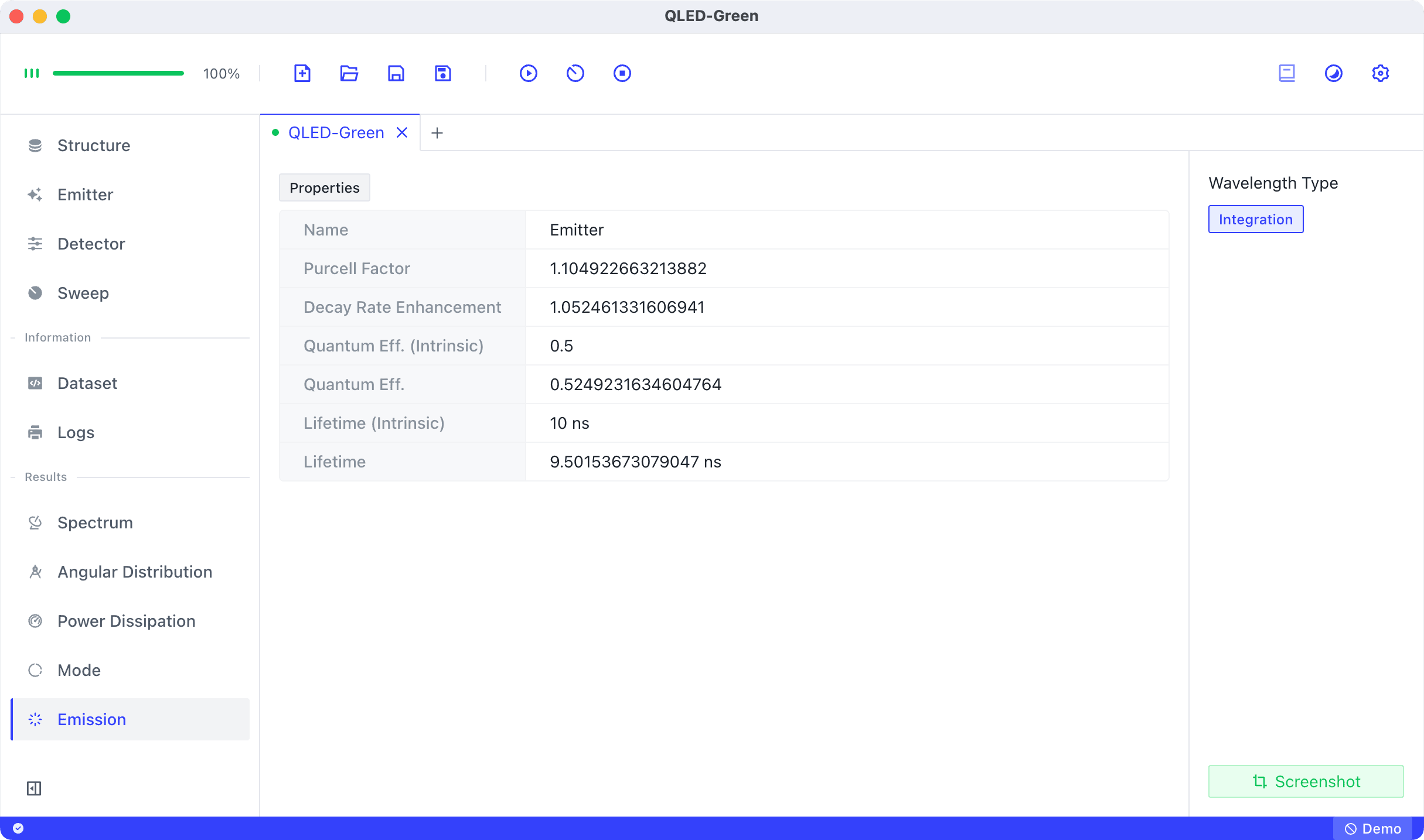
A Purcell Factor greater than 1 indicates enhanced spontaneous emission, with an effective quantum efficiency Quantum Eff. of 52.5%, higher than the intrinsic quantum efficiency Quantum Eff. (Intrinsic) of 50%. In the future, we can significantly increase the Purcell Factor through microcavity design to achieve further improvements in effective quantum efficiency.

Purcell factor is wavelength-dependent. Set the Mode detector’s Wavelength Type to Sweep to obtain the following results.

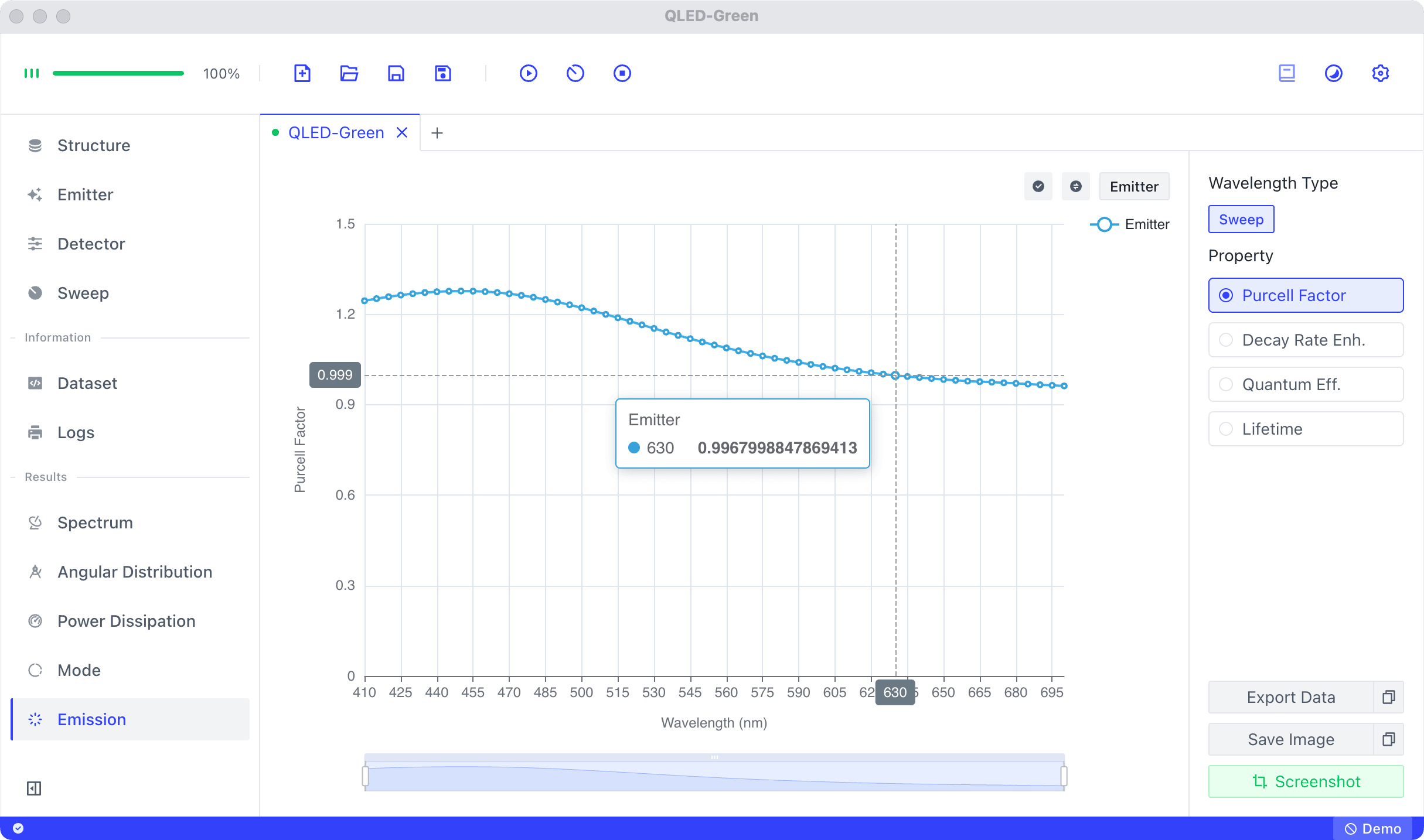
The maximum Purcell factor of 1.277 occurs at 450 nm, then continuously decreases. When the wavelength exceeds 630 nm, the Purcell factor is less than 1, indicating suppressed spontaneous emission.